Recurrent Neural Network
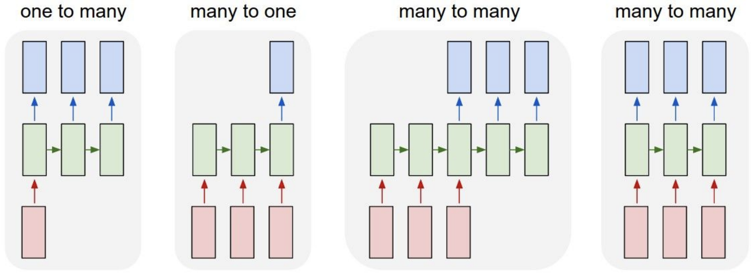
Recurent Network의 종류들 :
-
One to many :
Ex. Image Captioning : 이미지를 묘사하는 단어들의 sequence를 출력
-
Many to one :
Ex. Sentiment Classification : 단어들로 구성된 sequence(트위터 메세지 같은 것)를 입력으로 넣어 감정을 분류함
-
Many to many :
Ex. Machine Translation : 영어단어로 구성된 문장이 들어왔을 때, 한국어 단어로 구성된 문장으로 번역
-
Many to many :
Ex. Video Classification on frame level : 비디오에서 frame하나하나를 classification을 함
- 예측이 현재 시점의 frame에 국한되면 안됨
- 비디오 예측은 현재 시점의 frame과 현재 시점 전에 지나간 모든 frame들에 대한 함수가 되어야됨
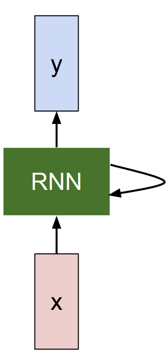
RNN의 과정
-
x : input vector
-
RNN :
-
내부적으로 state를 가짐
-
state를 function으로 변형 시킬 수 있음
-
Weight로 구성되며 Weight들이 튜닝되어감에 따라서 RNN이 진화되어나가기 때문에, 새로운 input이 들어올때 마다 다른 반응을 보임
-
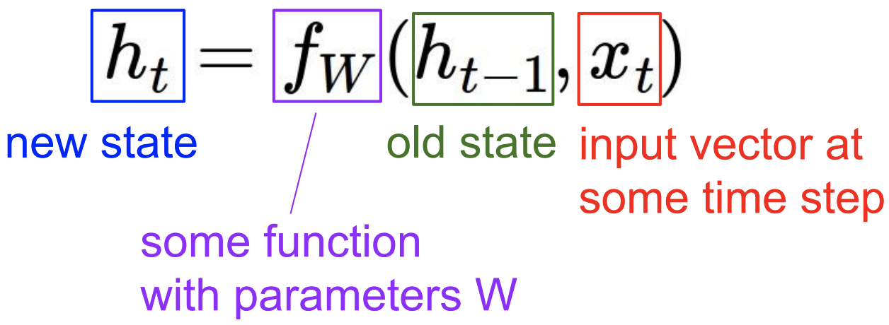
매 time step 마다 입력되는 vector에 대해서 recurrence function을 적용할 수 있음. recurrence function을 적용함으로써 sequence를 처리해 줄 수 있게됨 :
-
State : Vector의 collection
 모든 time step에서 동일한 recurrence function 과 동일한 parameter가 사용됨
-
-
-
y : 우리는 특정 time step에서의 vector의 예측을 원함
Example. RNN에게 Character sequence (“hello”) 를 feeding을 시키고 매 순간의 time step에서 RNN에게 다음 step에 어떤 Character가 와야되는지 묻는 것
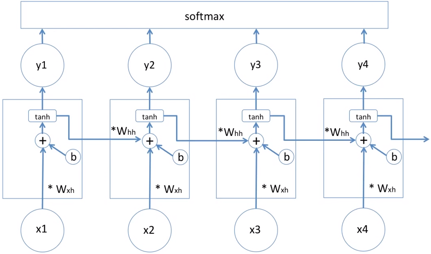
- W_hh : hidden 에서 hidden으로 이동하는 weight
- W_xh : x에서 hidden으로 이동하는 weight
- W_hy : hidden 에서 y으로 이동하는 weight
Implementation using NumPy
Data Input/Output
import numpy as np

data = open('input.txt', 'r').read() # should be simple plain text file
chars = list(set(data))
data_size, vocab_size = len(data), len(chars)
print 'data has %d characters, %d unique.' % (data_size, vocab_size)
char_to_ix = { ch:i for i,ch in enumerate(chars) }
ix_to_char = { i:ch for i,ch in enumerate(chars) }
-
enumerate(): index 번호와 list의 원소를 tuple형태로 return함>>> t = [1, 5, 7, 33, 39, 52] >>> for p in enumerate(t): ... print(p) ... (0, 1) (1, 5) (2, 7) (3, 33) (4, 39) (5, 52)
Initialization
# hyperparameters
hidden_size = 100 # size of hidden layer of neurons
seq_length = 25 # number of steps to unroll the RNN for
learning_rate = 1e-1 #10^(-1)

# model parameters
Wxh = np.random.randn(hidden_size, vocab_size)*0.01 # input to hidden
Whh = np.random.randn(hidden_size, hidden_size)*0.01 # hidden to hidden
Why = np.random.randn(vocab_size, hidden_size)*0.01 # hidden to output
bh = np.zeros((hidden_size, 1)) # hidden bias
by = np.zeros((vocab_size, 1)) # output bias
-
seq_length: 입력된 sequence의 길이 제약을 둬서 일괄 처리 할 수 있는 숫자를 나타냄
Main loop
n, p = 0, 0
mWxh, mWhh, mWhy = np.zeros_like(Wxh), np.zeros_like(Whh), np.zeros_like(Why)
mbh, mby = np.zeros_like(bh), np.zeros_like(by) # memory variables for Adagrad
smooth_loss = -np.log(1.0/vocab_size)*seq_length # loss at iteration 0
while True:
  # input 준비 과정
  if p+seq_length+1 >= len(data) or n == 0:
    hprev = np.zeros((hidden_size,1)) # reset RNN memory
    p = 0 # go from start of data
  inputs = [char_to_ix[ch] for ch in data[p:p+seq_length]]
  targets = [char_to_ix[ch] for ch in data[p+1:p+seq_length+1]]

  # sample() 호출 함으로 써 학습의 매 time step 마다 예측하는 character를 output으로 출력
  if n % 100 == 0:
    sample_ix = sample(hprev, inputs[0], 200)
    txt = ''.join(ix_to_char[ix] for ix in sample_ix)
    print '----\n %s \n----' % (txt, )

  # Network를 통해 25개 character를 forward 시킨 다음 loss 값 구하기
  loss, dWxh, dWhh, dWhy, dbh, dby, hprev = lossFun(inputs, targets, hprev)
  smooth_loss = smooth_loss * 0.999 + loss * 0.001
  if n % 100 == 0: print 'iter %d, loss: %f' % (n, smooth_loss) # print progress

  # parameter 업데이트
  for param, dparam, mem in zip([Wxh, Whh, Why, bh, by],
                                [dWxh, dWhh, dWhy, dbh, dby],
                                [mWxh, mWhh, mWhy, mbh, mby]):
    mem += dparam * dparam
    param += -learning_rate * dparam / np.sqrt(mem + 1e-8) # adagrad update

  p += seq_length # move data pointer
  n += 1 # iteration counter
-
hprev: 전 단계의 hidden state vector- hidden state vector가 batch에서 batch로 이어질 때 잘 porpagation이 될 수 있도록 하는 것
Loss Function
def lossFun(inputs, targets, hprev):
  """
  inputs : list of integers
  targets : list of integers
  hprev : Hx1 array of initial hidden state
  return : the loss, gradients on model parameters, and last hidden state
  """
  xs, hs, ys, ps = {}, {}, {}, {}
  hs[-1] = np.copy(hprev)
  loss = 0

  # forward pass
  for t in xrange(len(inputs)): # 25번 반복
    xs[t] = np.zeros((vocab_size,1)) # input 부분 one-hot encoding 하기
    xs[t][inputs[t]] = 1 						 # input 부분 one-hot encoding 하기
    hs[t] = np.tanh(np.dot(Wxh, xs[t]) + np.dot(Whh, hs[t-1]) + bh)
    ys[t] = np.dot(Why, hs[t]) + by
    ps[t] = np.exp(ys[t]) / np.sum(np.exp(ys[t]))
    loss += -np.log(ps[t][targets[t],0])

  # backward pass: compute gradients going backwards
  dWxh, dWhh, dWhy = np.zeros_like(Wxh), np.zeros_like(Whh), np.zeros_like(Why)
  dbh, dby = np.zeros_like(bh), np.zeros_like(by)
  dhnext = np.zeros_like(hs[0])
  for t in reversed(xrange(len(inputs))):  # 25부터 1까지
    dy = np.copy(ps[t])
    dy[targets[t]] -= 1 # backprop into y.
    dWhy += np.dot(dy, hs[t].T)
    dby += dy
    dh = np.dot(Why.T, dy) + dhnext # backprop into h
    dhraw = (1 - hs[t] * hs[t]) * dh # backprop through tanh nonlinearity
    dbh += dhraw
    dWxh += np.dot(dhraw, xs[t].T)
    dWhh += np.dot(dhraw, hs[t-1].T)
    dhnext = np.dot(Whh.T, dhraw)

  for dparam in [dWxh, dWhh, dWhy, dbh, dby]:
    np.clip(dparam, -5, 5, out=dparam) # clip to mitigate exploding gradients
  return loss, dWxh, dWhh, dWhy, dbh, dby, hs[len(inputs)-1]
-
forward pass
-
hs[t]: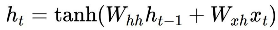
-
ys[t]: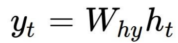
-
ps[t]: Softmax function -
loss: Cross entropy loss
-
-
np.clip(): -5와 5를 넘어서면 이 범위 안에 들어오도록 clipping 해줌>>> a = np.arange(10) >>> a array([0, 1, 2, 3, 4, 5, 6, 7, 8, 9]) >>> np.clip(a, 3, 6, out=a) array([3, 3, 3, 3, 4, 5, 6, 6, 6, 6]) >>> a array([3, 3, 3, 3, 4, 5, 6, 6, 6, 6])- RNN에서는 Gradient가 exploding되는 단점을 지니고 있기 때문에 사용됨
Sample
def sample(h, seed_ix, n):
  """
  RNN이 training에서 학습한 것과 character들이 통계에 기반하여서 새로운 text 데이터를 생성하도록 하는 함수
  h : memory state
  seed_ix : seed letter for first time step
  """
  x = np.zeros((vocab_size, 1)) # 입력값 one-hot encoding
  x[seed_ix] = 1								# 입력값 one-hot encoding
  ixes = []
  for t in xrange(n):
    h = np.tanh(np.dot(Wxh, x) + np.dot(Whh, h) + bh)
    y = np.dot(Why, h) + by
    p = np.exp(y) / np.sum(np.exp(y))
    ix = np.random.choice(range(vocab_size), p=p.ravel())
    x = np.zeros((vocab_size, 1)) # 결과값 one-hot encoding
    x[ix] = 1											# 결과값 one-hot encoding
    ixes.append(ix)
  return ixes
-
h:
-
y:
-
p: Softmax function
Experiment
- 생성된 C 코드에서 Syntax error문제들( 변수 선언하고 끝까지 사용하지 않음, 변수 선언 안하고 사용 등)은 존재함
- 그래도 상당히 흡사한 코드를 생성함
RNN 응용
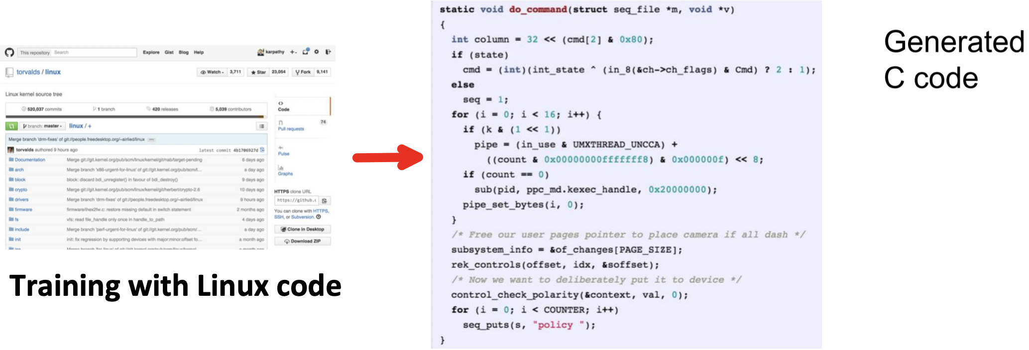
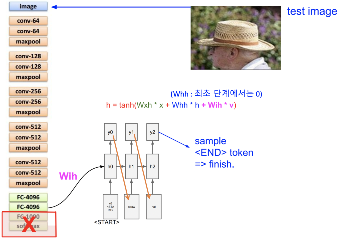
Image Captioning
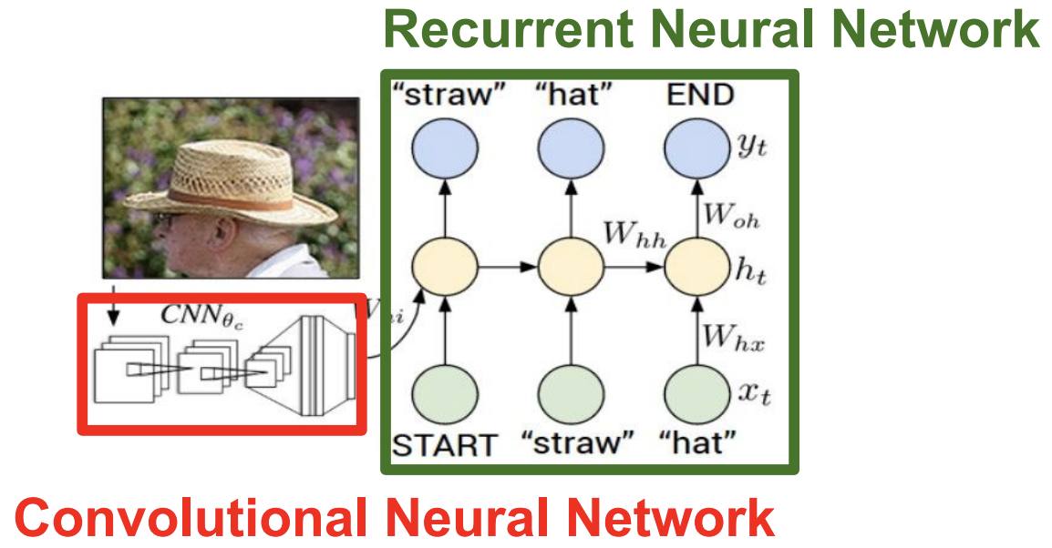
- CNN : image를 처리
- RNN : sequence를 처리
- CNN의 결과물(Classification을 한 결과)를 입력값으로 받아서 어떤걸 출력하는 방식
- CNN + RNN 하나의 단일 모델이라서 backpropagation은 한꺼번에 진행됨
-
처음에 CNN부분 에서 image를 입력으로 넣고 , 마지막에 FC를 softmax하지 않고 4096 dim vector 그대로 출력함
- Image Captioning에서는 다음 단어를 예측하는일, 이미지 정보를 기억하는 일이 병행해야됨
-
Example.
- CNN이 image에서 밀집(“straw”)을 인식하고 h0의 state에 영향을 주게됨
- 그럼 h0에서 y0으로 전달 할 때, “straw” 관련된 특정 수치가 높아지게됨
-
Example.
-
만약 x를 300 차원으로 표현했으면, y는 301차원을 가지게 됨 (End Token이 들어가기 때문에)
- 이 모델을 학습시키기 위해서는 natural language caption이 있는 이미지를 가지고 있어야 한다 (Microsoft COCO dataset)
- 한계점 : RNN은 전체 image를 딱 한번만 보고 끝남
Attention
-
이 모델은 이미지의 다양한 부분을 보면서 caption을 생성한다
-
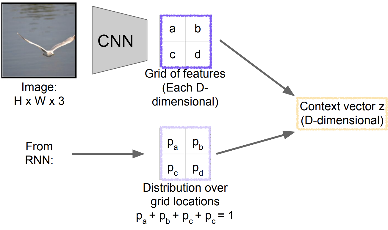
Soft Attention for Captioning

-
image를 CNN에 넣어주고 feature grid을 추출함
(feature grid : D 차원의 activation map)
-
feature grid를 첫번째 hidden state를 초기화하는데 사용되고 이를 통해 a1이라는 걸 추출함
(a1 : 위치에 대한 확률 분포)
-
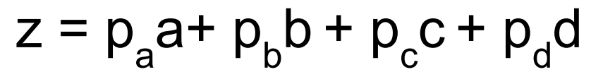
a1를 feature grid와 연산을 해서 weighted feature를 구하게 됨
(weighted feature : input 이미지를 summerize하는 vector)
-
weighted feature를 구하는 2가지 방법 :
-
Soft attention
- 모든 location(grid)을 고려 :
- 장점 : backprop이 가능함으로 End-to-End 훈련가능
- 단점 : 모든 grid를 고려함으로 Hard attention 보다 연산량이 많음
- 모든 location(grid)을 고려 :
-
Hard attention
-
가장 높은 확률을 가지는 grid를 선택 :
Example. Pa가 가장 높은 확률을 가진다면 이 쪽 영역을 선택해서 argmax를 통해 이쪽 영역의 feature vector의 요소를 추출하게 됨
-
장점 : Soft attention보다 연산량이 적고 정확도가 좀더 높음
-
단점 : backprop이 안되서 별도의 강화 학습을 시켜줘야 됨
-
-
-
Soft attention
 Hard attention
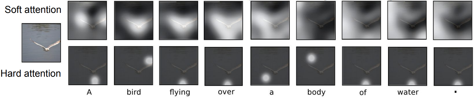
 관찰Point - 모델이 스스로 더 적합한 captioning을 하기 위해 다음에 attention을 줄 부분을 결정함
💁🏻 Soft attention : 모든 위치를 고려하고 모든 위치들의 확률을 평균했기 때문에 diffusion한 효과가 남. 즉, 확률분포를 시각화한 셈
💁🏻 Hard attention : 최대 확률을 보이는 한군데 위치만 고려하기 때문에 한 군데만 밝게 보임
-
-
weighted feature vector, 첫번째 단어, 이전 단계의 hidden state 가 입력으로 들어가서 h1을 생성하게 됨
-
h1은 d1과 a2를 output으로 냄
(d1 : 단어에 대한 확률 분포)
(a2 : 위치에 대한 확률 분포)
-
a2를 가지고 다시 3. 부터 진행되는 반복
-
-
Attention 매커니즘의 한계점 : Fixed grid에 한정되어서 attention을 주게 됨
-
임의 지점의 Attention을 주는 방법들 :
-
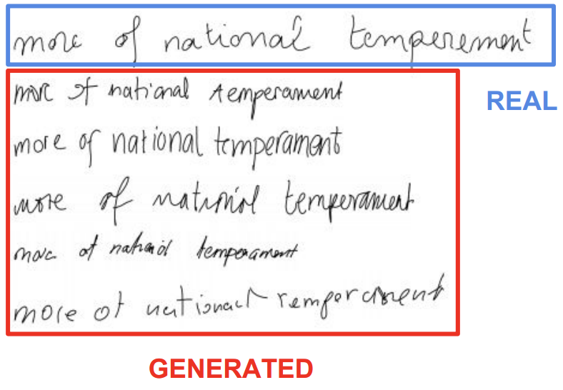
Graves, “Generating Sequences with Recurrent Neural Networks”, arXiv 2013
-
Text를 읽은 다음에 실제 손글씨 처럼 Text를 생성해줌
-
-
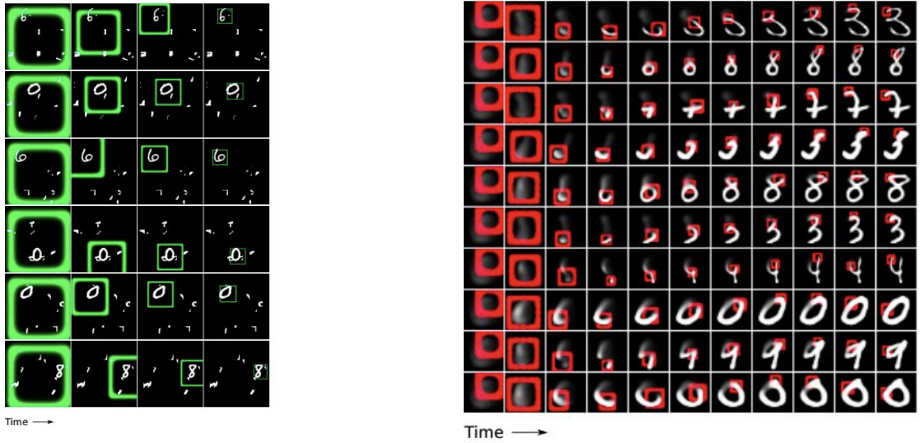
Gregor et al, “DRAW: A Recurrent Neural Network For Image Generation”, ICML 2015
-
input에 있어서 임의 지점에 Attention을 주면서 image classify 가능, output에 있어서도 임의 지점에 Attention을 주면서 image를 생성 해냄
-
-
Jaderberg et al, “Spatial Transformer Networks”, NIPS 2015
-
DRAW와 비슷하면서 좀 더 체계화 됨
-
Question : input 이미지에서 object localize를 해서 Box에 대한 좌표가 생기고 이 좌표를 기반으로 crop하고 rescaling을 하는 과정을 미분 가능한 함수로 만들 수 있는가?
🤔 output의 pixel 좌표를 input의 pixel 좌표에 mapping을 시켜주는 함수를 만들어주자
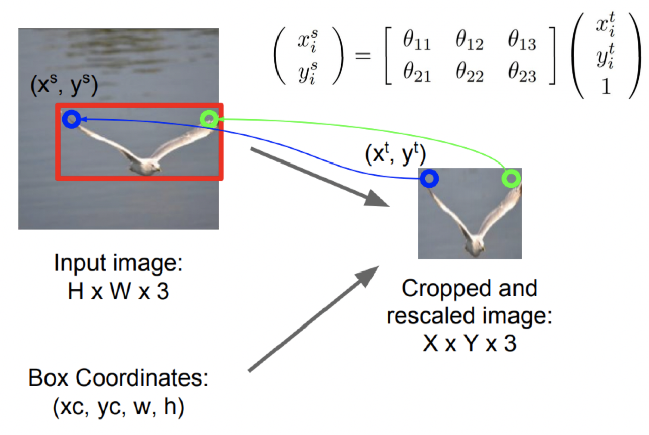
output의 한 좌표가 input 이미지에 어디에 mapping 되는지 이것을 찾는 과정을 반복함
우리 network는 θ들을 예측하면서 input에 attention을 주게됨
-
Spatial Transformer Networks의 전체 과정이 연속적이고 미분 가능함
-
전체 pipeline
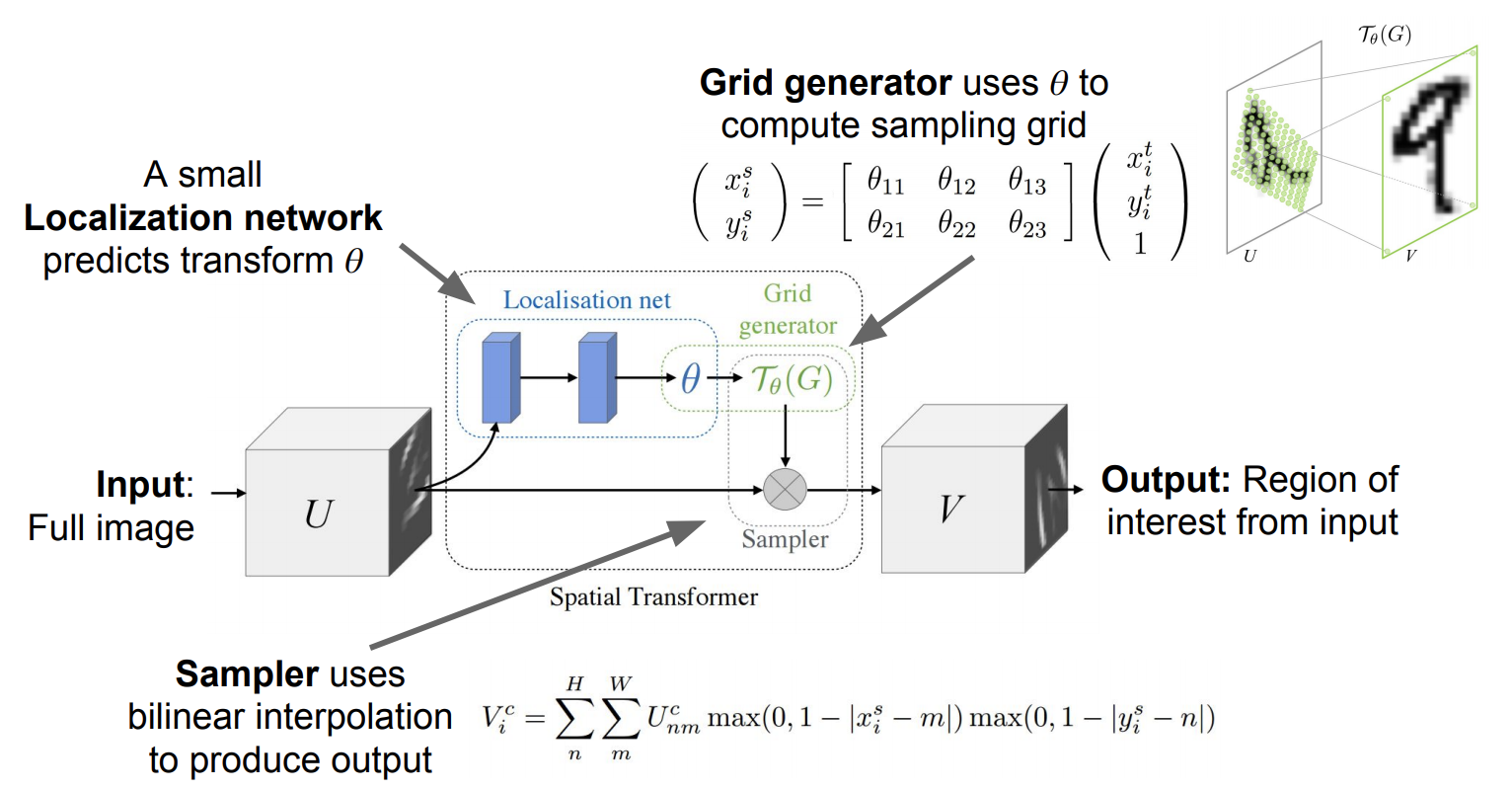
- Input feature map U가 Localization net에 들어가서 transformation parameter θ를 뽑아냄
- 이때 Localization net의 구조는 conv. net 이든 FC net이든 상관없이 마지막에 Regression layer만 잘 들어가서 parameter 추출만 잘하면 됨
- 앞에서 뽑아낸 transformation parameter θ는 grid generator에 들어가서 sampling 지점의 위치가 지정된 sampling grid Tθ(G) 를 생성함
- Sampler에는 Input feature map U와 sampling grid Tθ(G)가 입력으로 들어감
- sampling grid Tθ(G)에는 sampling point가 찍혀있기 때문에 그것을 Input feature map U에 적용하면 output feature map V를 뽑아낼 수 있음
- Input feature map U가 Localization net에 들어가서 transformation parameter θ를 뽑아냄
-
결과물
-
Spatial Transformer는 동적으로 각각에 맞는 transformation을 해줌
-
차원이 꼬여있는 것들에 대해서 입체적으로 분석해서 제대로 된 결과를 도출함
-
회전된 이미지에 대해서도 잘 복원을 해줌
-
Spatial Transformer를 잘 갖추게된다면 일반적인 Classification Network에 삽입을 해주고 attention을 주는 법을 학습하게 해줄수 있게 됨
-
spatial invariance : 이미지가 변환되어도 그 이미지로 인식하는 것. (ex. 고양이를 90도 회전시켜놓아도 고양이로 인식하는 능력)
-
이미지 분류 문제에서는 spatial invariance 가 중요한데 일반적인 CNN에서는 이를 해결하기 위해 max pooling layer가 필요함
-
Spartial Transformation은 max pooling layer보다 더 좋은 spatial invariance 능력을 갖게 하기 위해 이미지의 특정 부분을 자르고 변환해서 그 부분만 떼어서 트레이닝을 시킴
-
이 변환하는 과정을 affine transformation이라고 함
-
CNN 안에 하나의 layer로 spartial transformation module이 들어가는데 이 layer는 위의 affine transformation을 하는데 필요한 parameter을 배움
-
CNN 입력 바로 앞에 Spatial Transformer Layer를 두는 것이 👍
-
-
-
-
Long Short Term Memory (LSTM)
- RNN은 입력 squence 길이가 길어지면 오래된 데이터를 잊어버리는 치명적인 단점이 있음
- 위 그림은 입력 squence 길이가 짧아서 문제는 없지만 만약 입력 squence 길이가 100개 이상일 경우 다음과같은 문제들이 생긴다
-
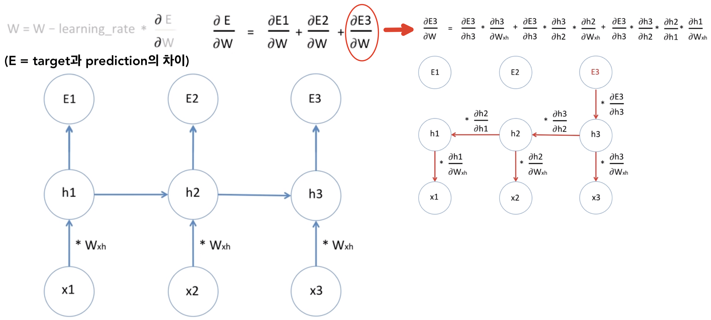
Vanishing Gradient :
backpropagation时 Gradient (
 )가 0에 근접하면 새로 업데이트 되는 Weight는 기존의 Weight와 별 차이가 없어짐 💁🏻 즉, 학습시간이 길어지고 비효율적임
 -
Exploding Gradient
backpropagation时 Gradient (
)가 매우 큰 수가 되어 새로 업데이트 되는 Weight는 기존의 Weight와 매우 다르게 업데이트됨 💁🏻 즉, 이후 Weight의 업데이트의 변화가 커지면서 훈련이 수렴되지 못함
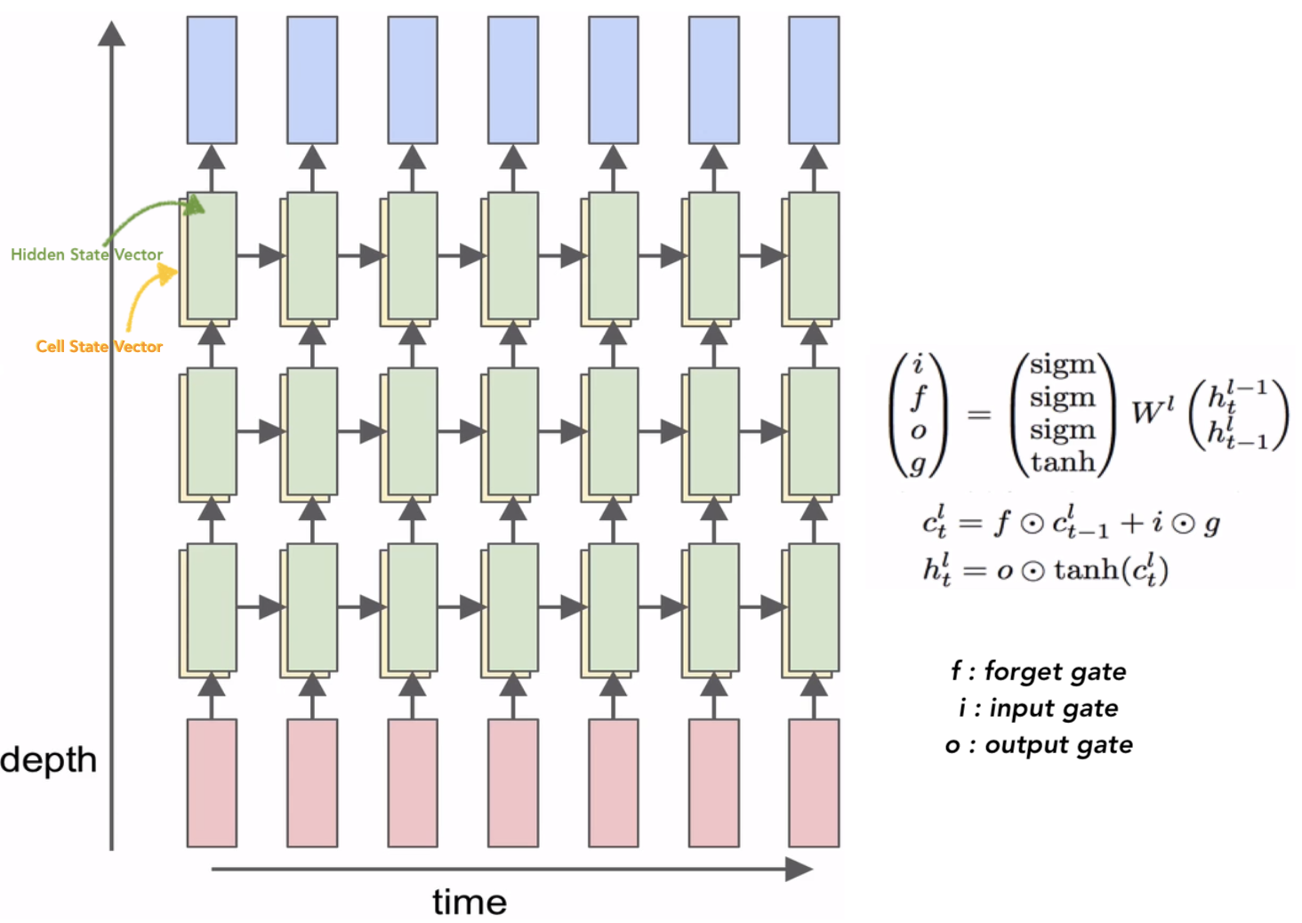
- LSTM은 기존 RNN의 hidden state 이외에도 별도의 cell state라는 변수(variable)를 두어, 그 기억력을 증가시켰을 뿐만 아니라, 여러가지 게이트(gate)를 두어 기억하거나, 잊어버리거나, 출력하고자 하는 데이터의 양을 상황에 따라서, 마치 수도꼭지를 잠궜다 열듯이, 효과적으로 제어하여 긴 길이의 데이터에 대해서도 효율적으로 대처할 수 있게 되었음
-
현재의 cell state 구하기 :
- f : 현재의 cell state가 바로 그 전의 cell state를 얼마나 잊을 것이냐 를 정해주는 것
- g : input 값을 현재의 cell state에 얼마나 더해주거나 빼줄 것이냐 를 정해주는 것
-
현재의 hidden state 구하기 :
- 현재의 cell state에 tanh를 취해준 다음 o를 곱해줌
- o : 현재의 cell state 중에 어느 부분을 다음의 hidden cell로 전달할 지 결정하는 것
- LSTM는 vanishing gradient 문제를 해결함?
- LSTM doesn’t guarantee that there is no vanishing/exploding gradient
- but it does provide an easier way for the model to learn long-distance dependencies
- LSTM doesn’t guarantee that there is no vanishing/exploding gradient
-
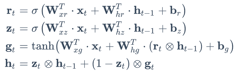
LSTM의 확장판 : Gated Recurrent Unit (GRU)
-
LSTM 셀의 간소화된 버전
-
두 상태 벡터 cell state 와 hidden state가 하나의 hidden state vector로 합쳐짐
-
하나의 gate controller인 z가 forget과 input gate를 모두 제어함
-
GRU cell은 output gate가 없어 전체 state vector가 time step마다 출력되며, 이전 hidden state vector의 어느 부분이 출력될지 제어하는 새로운 gate controller인 r 이 있음
-
《Reference》